pacman::p_load(jsonlite, tidyverse, ggtext,
                knitr, lubridate, patchwork,
                ggraph, tidygraph, igraph, scales,
ggiraph, dplyr, stringr, ggnewscale)Take-home Exercise 2
Take-home Exercise
1 Overview
This take-home exercise will be done in reference to the VAST Challenge 2025 and provide solutions to the first question of Mini-Challenge 1.
1.1 Background
One of music’s biggest superstars is Oceanus native Sailor Shift. From humble beginnings, Sailor has grown in popularity and now enjoys fans around the world. Sailor started her career on the island nation of Oceanus which can be clearly seen in her early work, she started in the genre of “Oceanus Folk”. While Sailor has moved away from the traditional Oceanus style, the Oceanus Folk has made a name for itself in the musical world. The popularity of this music is one of the factors driving an increase in tourism to a quiet island nation that used to be known for fishing.
In 2023, Sailor Shift joined the Ivy Echoes – an all-female Oceanus Folk band consisting of Sailor (vocalist), Maya Jensen (vocalist), Lila “Lilly” Hartman (guitarist), Jade Thompson (drummer), and Sophie Ramirez (bassist). They played together at venues throughout Oceanus but had broken up to pursue their individual careers by 2026. Sailor’s breakthrough came in 2028 when one of her singles went viral, launched to the top of the global charts (something no other Oceanus Folk song had ever done). Since then, she has only continued to grow in popularity worldwide.
Sailor has released a new album almost every year since her big break, and each has done better than the last. Although she has remained primarily a solo artist, she has also frequently collaborated with other established artists, especially in the Indie Pop and Indie Folk genres. She herself has branched out musically over the years but regularly returns to the Oceanus Folk genre — even as the genre’s influence on the rest of the music world has spread even more.
Sailor has always been passionate about two things: (1) spreading Oceanus Folk, and (2) helping lesser-known artists break into music. Because of those goals, she’s particularly famous for her frequent collaborations.
Additionally, because of Sailor’s success, more attention began to be paid over the years to her previous bandmates. All 4 have continued in the music industry—Maya as an independent vocalist, Lilly and Jade as instrumentalists in other bands, and Sophie as a music producer for a major record label. In various ways, all of them have contributed to the increased influence of Oceanus folk, resulting in a new generation of up-and-coming Oceanus Folk artists seeking to make a name for themselves in the music industry.
Now, as Sailor returns to Oceanus in 2040, a local journalist – Silas Reed – is writing a piece titled Oceanus Folk: Then-and-Now that aims to trace the rise of Sailor and the influence of Oceanus Folk on the rest of the music world. He has collected a large dataset of musical artists, producers, albums, songs, and influences and organized it into a knowledge graph. Your task is to help Silas create beautiful and informative visualizations of this data and uncover new and interesting information about Sailor’s past, her rise to stardom, and her influence.
1.2 Tasks and Questions
The objective of this take-home exercise is to address the following tasks and questions of VAST Challenge 2025’s Mini-Challenge 1.
Design and develop visualizations and visual analytic tools that will allow Silas to explore and understand the profile of Sailor Shift’s career
Who has she been most influenced by over time?
Who has she collaborated with and directly or indirectly influenced?
How has she influenced collaborators of the broader Oceanus Folk community?
2 Getting Started
2.1 Load the packages
In the code chunk below, p_load() of pacman package is used to load the R packages into R environemnt.
2.2 Importing Knowledge Graph Data
fromJSON() of jsonlite package is used to import MC1_graph.json file into R and save the output object.
mc1_data <- fromJSON("MC1/data/MC1_graph.json")2.2.1 Inspect structure
Here, str() is used to reveal the structure of mc1_data object.
str(mc1_data, max.level = 1)List of 5
$ directed : logi TRUE
$ multigraph: logi TRUE
$ graph :List of 2
$ nodes :'data.frame': 17412 obs. of 10 variables:
$ links :'data.frame': 37857 obs. of 4 variables:2.3 Extracting the edges and nodes tables
Next, as_tibble() of tibble package package is used to extract the nodes and links tibble data frames from mc1_data object into two separate tibble data frames called mc1_nodes_raw and mc1_edges_raw respectively.
mc1_nodes_raw <- as_tibble(mc1_data$nodes)
glimpse(mc1_nodes_raw)
Rows: 17,412
Columns: 10
$ `Node Type` <chr> "Song", "Person", "Person", "Person", "RecordLabel", "S…
$ name <chr> "Breaking These Chains", "Carlos Duffy", "Min Qin", "Xi…
$ single <lgl> TRUE, NA, NA, NA, NA, FALSE, NA, NA, NA, NA, TRUE, NA, …
$ release_date <chr> "2017", NA, NA, NA, NA, "2026", NA, NA, NA, NA, "2020",…
$ genre <chr> "Oceanus Folk", NA, NA, NA, NA, "Lo-Fi Electronica", NA…
$ notable <lgl> TRUE, NA, NA, NA, NA, TRUE, NA, NA, NA, NA, TRUE, NA, N…
$ id <int> 0, 1, 2, 3, 4, 5, 6, 7, 8, 9, 10, 11, 12, 13, 14, 15, 1…
$ written_date <chr> NA, NA, NA, NA, NA, NA, NA, NA, NA, NA, "2020", NA, NA,…
$ stage_name <chr> NA, NA, NA, NA, NA, NA, NA, NA, NA, NA, NA, NA, NA, NA,…
$ notoriety_date <chr> NA, NA, NA, NA, NA, NA, NA, NA, NA, NA, NA, NA, NA, NA,…kable(head(mc1_nodes_raw, 5))| Node Type | name | single | release_date | genre | notable | id | written_date | stage_name | notoriety_date |
|---|---|---|---|---|---|---|---|---|---|
| Song | Breaking These Chains | TRUE | 2017 | Oceanus Folk | TRUE | 0 | NA | NA | NA |
| Person | Carlos Duffy | NA | NA | NA | NA | 1 | NA | NA | NA |
| Person | Min Qin | NA | NA | NA | NA | 2 | NA | NA | NA |
| Person | Xiuying Xie | NA | NA | NA | NA | 3 | NA | NA | NA |
| RecordLabel | Nautical Mile Records | NA | NA | NA | NA | 4 | NA | NA | NA |
mc1_edges_raw <- as_tibble(mc1_data$links)

glimpse(mc1_edges_raw)
Rows: 37,857
Columns: 4
$ `Edge Type` <chr> "InterpolatesFrom", "RecordedBy", "PerformerOf", "Composer…
$ source <int> 0, 0, 1, 1, 2, 2, 3, 5, 5, 5, 5, 5, 5, 5, 5, 5, 5, 5, 5, 5…
$ target <int> 1841, 4, 0, 16180, 0, 16180, 0, 5088, 14332, 11677, 2479, …
$ key <int> 0, 0, 0, 0, 0, 0, 0, 0, 0, 0, 0, 0, 0, 0, 0, 0, 0, 0, 0, 0…kable(head(mc1_edges_raw, 5))| Edge Type | source | target | key |
|---|---|---|---|
| InterpolatesFrom | 0 | 1841 | 0 |
| RecordedBy | 0 | 4 | 0 |
| PerformerOf | 1 | 0 | 0 |
| ComposerOf | 1 | 16180 | 0 |
| PerformerOf | 2 | 0 | 0 |
2.4 Data Overview
Before proceeding to data pre-processing, we examine the data to gain a clearer understanding of the dataset and to verify the structural integrity of the imported graph.
In this code chunk below, ggplot2 functions are used the reveal the frequency distribution of Node Type field of mc1_nodes_raw.
ggplot(data = mc1_nodes_raw,
       aes(y = `Node Type`)) +
  geom_bar()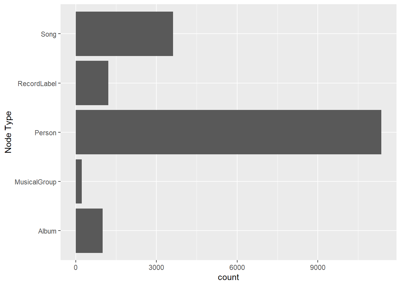
On the other hand, code chunk below uses ggplot2 functions to reveal the frequency distribution of Edge Type field of mc1_edges_raw.
ggplot(data = mc1_edges_raw,
       aes(y = `Edge Type`)) +
  geom_bar()
3 Data Pre-processing
3.1 Adding identifying columns
As a large part of this mini-challenge centers around Sailor Shift and the genre of “Oceanus Folk”, the following code will add columns to help with identification and filtering of Sailor Shift and the work in the genre of “Oceanus Folk”. This will help with analysis in addressing the questions and tasks.
mc1_nodes_raw <- mc1_nodes_raw %>%
  mutate(
    is_sailor = (
      str_detect(name, regex("sailor shift", ignore_case = TRUE))
    ) %>% replace_na(FALSE),

    is_oceanus_folk = str_detect(genre, regex("oceanus folk", ignore_case = TRUE)) %>% #na/not oceanus folk = false
      replace_na(FALSE)
  )
3.2 Converting date field
Date fields will be converted from chr to int for later analysis. Note that dates only appear for Song and Album.
mc1_nodes_raw <- mc1_nodes_raw %>%
  mutate(across(c(release_date, notoriety_date, written_date),
                ~as.integer(if_else(`Node Type` %in% c("Song", "Album"), ., NA_character_))))
3.3 Check for duplicates
3.3.1 Check for duplicates in mc1_nodes_raw
The following code chunk checks for id duplicates in mc1_nodes_raw.
mc1_nodes_raw %>%
  count(id) %>%
  filter(n > 1)
# A tibble: 0 × 2
# ℹ 2 variables: id <int>, n <int>There are no duplicated id in mc1_nodes_raw.
The following code checks for name duplicates in mc1_nodes_raw.
duplicated_name <- mc1_nodes_raw %>%
  count(name) %>%
  filter(n > 1)

duplicated_name
# A tibble: 1,611 × 2
name n
<chr> <int>
1 Agata Records 2
2 Ancestral Echoes 2
3 Angela Thompson 2
4 Anthony Davis 2
5 Anthony Smith 2
6 Asuka Takahashi 3
7 Brandon Wilson 2
8 Brian Gonzalez 2
9 Bryan Garcia 2
10 Bryan Smith 3
# ℹ 1,601 more rowsThe following code chunk shows all rows from mc1_nodes_raw that have duplicated names, and sorting them alphabetically by the name column. There are a total of 4,953 records with duplicated names in mc1_nodes_raw.
mc1_nodes_raw %>%
  filter(name %in% duplicated_name$name) %>%
  arrange(name)
# A tibble: 4,953 × 12
`Node Type` name single release_date genre notable id written_date
<chr> <chr> <lgl> <int> <chr> <lgl> <int> <int>
1 RecordLabel Agata Recor… NA NA <NA> NA 1528 NA
2 RecordLabel Agata Recor… NA NA <NA> NA 17388 NA
3 Song Ancestral E… TRUE 1991 Drea… FALSE 11793 NA
4 Song Ancestral E… FALSE 2039 Avan… TRUE 17133 NA
5 Person Angela Thom… NA NA <NA> NA 1150 NA
6 Person Angela Thom… NA NA <NA> NA 13448 NA
7 Person Anthony Dav… NA NA <NA> NA 8692 NA
8 Person Anthony Dav… NA NA <NA> NA 12452 NA
9 Person Anthony Smi… NA NA <NA> NA 5719 NA
10 Person Anthony Smi… NA NA <NA> NA 7694 NA
# ℹ 4,943 more rows
# ℹ 4 more variables: stage_name <chr>, notoriety_date <int>, is_sailor <lgl>,
# is_oceanus_folk <lgl>3.3.2 Fixing duplicates in mc1_nodes_raw
The section will focus on fixing the duplicates found in mc1_nodes_raw as identified in section 3.3.1.
The following code chunk will tag each row with a unique key (group_key) based on its respective column values. This helps to identify unique records.
# Step 1: Mark all node rows with a hash key for grouping
mc1_nodes_tagged <- mc1_nodes_raw %>%
  mutate(group_key = paste(`Node Type`, name, single, release_date, genre,
                           notable, written_date, notoriety_date, is_sailor,
                           is_oceanus_folk, sep = "|"))

mc1_nodes_tagged
# A tibble: 17,412 × 13
`Node Type` name single release_date genre notable id written_date
<chr> <chr> <lgl> <int> <chr> <lgl> <int> <int>
1 Song Breaking Th… TRUE 2017 Ocea… TRUE 0 NA
2 Person Carlos Duffy NA NA <NA> NA 1 NA
3 Person Min Qin NA NA <NA> NA 2 NA
4 Person Xiuying Xie NA NA <NA> NA 3 NA
5 RecordLabel Nautical Mi… NA NA <NA> NA 4 NA
6 Song Unshackled … FALSE 2026 Lo-F… TRUE 5 NA
7 Person Luke Payne NA NA <NA> NA 6 NA
8 Person Xiulan Zeng NA NA <NA> NA 7 NA
9 Person David Frank… NA NA <NA> NA 8 NA
10 RecordLabel Colline-Cas… NA NA <NA> NA 9 NA
# ℹ 17,402 more rows
# ℹ 5 more variables: stage_name <chr>, notoriety_date <int>, is_sailor <lgl>,
# is_oceanus_folk <lgl>, group_key <chr>The code below deduplicates the dataset using group_key, reducing the number of duplicated names from 4,953 to 14. The remaining 14 names appear more than once because their corresponding records differ in at least one column used to form group_key, so they are retained as distinct entries.
# Step 2: Deduplicate and keep the preferred (with stage_name if available)
mc1_nodes_dedup <- mc1_nodes_tagged %>%
  group_by(group_key) %>%
  arrange(desc(!is.na(stage_name))) %>%
  slice(1) %>%
  ungroup()

duplicated_name <- mc1_nodes_dedup %>%
  count(name) %>%
  filter(n > 1)

mc1_nodes_raw %>%
  filter(name %in% duplicated_name$name) %>%
  arrange(name)
# A tibble: 14 × 12
`Node Type` name single release_date genre notable id written_date
<chr> <chr> <lgl> <int> <chr> <lgl> <int> <int>
1 Song Ancestral E… TRUE 1991 Drea… FALSE 11793 NA
2 Song Ancestral E… FALSE 2039 Avan… TRUE 17133 NA
3 RecordLabel Coastal Ech… NA NA <NA> NA 4022 NA
4 Album Coastal Ech… NA 2023 Psyc… TRUE 15065 2019
5 Song Postcards f… TRUE 2023 Indi… TRUE 12852 2023
6 Song Postcards f… FALSE 1984 Acou… FALSE 17214 NA
7 Album Shattered R… NA 2013 Emo/… TRUE 3325 2013
8 Song Shattered R… FALSE 2036 Dark… TRUE 17088 NA
9 Song Unheard Fre… TRUE 2025 Alte… TRUE 7999 NA
10 RecordLabel Unheard Fre… NA NA <NA> NA 10952 NA
11 Song Vanishing P… TRUE 2018 Avan… TRUE 9371 2018
12 Song Vanishing P… FALSE 2013 Ocea… FALSE 17338 NA
13 RecordLabel Vertical Ho… NA NA <NA> NA 2453 NA
14 Album Vertical Ho… NA 2017 Doom… TRUE 9262 NA
# ℹ 4 more variables: stage_name <chr>, notoriety_date <int>, is_sailor <lgl>,
# is_oceanus_folk <lgl>3.3.3 Check for duplicates in mc1_edges_raw
The following code proceeds to check for duplicates in mc1_edges_raw.
# Step 1: Identify duplicate combinations
duplicate_summary <- mc1_edges_raw %>%
  count(source, target, `Edge Type`) %>%
  filter(n > 1)

# Step 2: Join back to get all original duplicate rows
mc1_edges_raw %>%
  inner_join(duplicate_summary, by = c("source", "target", "Edge Type"))
# A tibble: 6 × 5
`Edge Type` source target key n
<chr> <int> <int> <int> <int>
1 PerformerOf 17057 17058 0 2
2 PerformerOf 17057 17058 1 2
3 PerformerOf 17349 17350 0 2
4 PerformerOf 17349 17350 2 2
5 PerformerOf 17355 17356 0 2
6 PerformerOf 17355 17356 2 2There are duplicates as seen above, with only differences in key. As key will not be used in subsequent data analysis, the duplicated edges will be removed with the following code.
mc1_edges_raw <- mc1_edges_raw %>%
  distinct(source, target, `Edge Type`, .keep_all = TRUE) %>%
  select(!key)

mc1_edges_raw %>%
  count(source, target, `Edge Type`) %>%
  filter(n > 1)
# A tibble: 0 × 4
# ℹ 4 variables: source <int>, target <int>, Edge Type <chr>, n <int>4 EDA
4.1 Explore and inspect Nodes
mc1_nodes_raw$release_date %>% unique() [1] 2017 NA 2026 2020 2027 2022 2007 2010 2003 2023 1997 2013 2000 2025 2029
[16] 2015 2018 2016 2014 2028 2021 2030 2011 1994 2004 1998 1991 1999 2024 2012
[31] 2002 2006 2008 2019 1995 1989 2032 2009 2001 1996 1990 1984 2005 1993 1986
[46] 1985 1981 1992 1987 1988 1983 2031 1975 2035 2033 2037 2036 2039 2038 2034
[61] 1977 1979 1980 1982 2040mc1_nodes_raw %>%
filter(grepl("Sailor Shift", name)) #Sailor Shift is in name column and not in stage_name column# A tibble: 1 × 12
`Node Type` name single release_date genre notable id written_date
<chr> <chr> <lgl> <int> <chr> <lgl> <int> <int>
1 Person Sailor Shift NA NA <NA> NA 17255 NA
# ℹ 4 more variables: stage_name <chr>, notoriety_date <int>, is_sailor <lgl>,
# is_oceanus_folk <lgl>' will be removed from name to prevent issues with tooltip in tidygraph.
mc1_nodes_clean <- mc1_nodes_raw %>%
  mutate(
    name = gsub("'", "", name))

kable(head(mc1_nodes_clean))| Node Type | name | single | release_date | genre | notable | id | written_date | stage_name | notoriety_date | is_sailor | is_oceanus_folk |
|---|---|---|---|---|---|---|---|---|---|---|---|
| Song | Breaking These Chains | TRUE | 2017 | Oceanus Folk | TRUE | 0 | NA | NA | NA | FALSE | TRUE |
| Person | Carlos Duffy | NA | NA | NA | NA | 1 | NA | NA | NA | FALSE | FALSE |
| Person | Min Qin | NA | NA | NA | NA | 2 | NA | NA | NA | FALSE | FALSE |
| Person | Xiuying Xie | NA | NA | NA | NA | 3 | NA | NA | NA | FALSE | FALSE |
| RecordLabel | Nautical Mile Records | NA | NA | NA | NA | 4 | NA | NA | NA | FALSE | FALSE |
| Song | Unshackled Heart | FALSE | 2026 | Lo-Fi Electronica | TRUE | 5 | NA | NA | NA | FALSE | FALSE |
4.2 Explore and inspect Edges
The following code chunk is used to ensure that id used in mc1_edges_raw matches the range range of id in mc1_nodes_clean.
range(mc1_nodes_clean$id)[1] 0 17411range(mc1_edges_raw$source)[1] 0 17411range(mc1_edges_raw$target)[1] 0 174114.3 Mapping Node name to Edges id
tidygraph uses from and to columns to reference nodes. By default, tidygraph matches these edges reference against the first column in the nodes table, or against name column.
Currently, source and target columns in mc1_edges_raw contain id values that correspond to the id column in mc1_nodes_clean. To properly integrate with tidygraph’s conventions, the following will be done:
- Restructure mc1_nodes_clean
- Rename the current name column to node_name - this is done to preserve the actual node names
- Rename the id column to name so it becomes the primary identifier column that tidygraph will use for matching
- Rename source and target columns in mc1_edges_raw, as required by tidygraph
- Ensure data type consistency: Convert the name column (formerly id) to character format to match the data type of the edge references
mc1_nodes_clean <- mc1_nodes_dedup %>%
  rename(node_name = name, name = id) %>%
  mutate(name = as.character(name)) %>%
  select(`Node Type`, node_name, release_date, genre, notable, name, single, written_date, stage_name, notoriety_date, is_sailor, is_oceanus_folk)

mc1_nodes_clean
# A tibble: 14,077 × 12
`Node Type` node_name release_date genre notable name single written_date
<chr> <chr> <int> <chr> <lgl> <chr> <lgl> <int>
1 Album A Lush Dyst… 2031 Psyc… TRUE 17005 NA 2030
2 Album Addicted to… 2004 Sout… TRUE 14658 NA 2000
3 Album Adriatic Em… 2013 Post… TRUE 10412 NA NA
4 Album Aerial Echo… 2023 Indi… TRUE 7908 NA NA
5 Album Aftershock … 2028 Drea… TRUE 2030 NA 2021
6 Album Allegretto … 2020 Indi… TRUE 6251 NA NA
7 Album Alleys and … 2029 Jazz… TRUE 1310 NA NA
8 Album Alloy Archi… 2017 Indi… TRUE 8428 NA 2017
9 Album Almost (But… 2027 Alte… TRUE 14611 NA 2027
10 Album Altar of De… 2020 Ocea… TRUE 5883 NA NA
# ℹ 14,067 more rows
# ℹ 4 more variables: stage_name <chr>, notoriety_date <int>, is_sailor <lgl>,
# is_oceanus_folk <lgl>4.3.1 Creating edge mapping from old id to kept id
In section 3.3.2, duplicated nodes were deduplicated and removed, edges referring to the removed nodes will become invalid thus, edges will be remapped to the retained nodes. This ensures that all edges correctly point to existing nodes in the deduplicated graph.
# Step 1: Create mapping of all group_key → kept id
key_to_id_map <- mc1_nodes_dedup %>%
  select(group_key, kept_id = id)

# Step 2: Map all original rows to the retained ID
id_remap <- mc1_nodes_tagged %>%
  left_join(key_to_id_map, by = "group_key") %>%
  select(original_id = id, kept_id)

id_remap
# A tibble: 17,412 × 2
original_id kept_id
<int> <int>
1 0 0
2 1 1
3 2 14470
4 3 3
5 4 4
6 5 5
7 6 6
8 7 7
9 8 8
10 9 9
# ℹ 17,402 more rows# Step 3: Replace edges' source and target with mapped kept_id
mc1_edges_mapped <- mc1_edges_raw %>%
left_join(id_remap, by = c("source" = "original_id"))
mc1_edges_mapped# A tibble: 37,854 × 4
`Edge Type` source target kept_id
<chr> <int> <int> <int>
1 InterpolatesFrom 0 1841 0
2 RecordedBy 0 4 0
3 PerformerOf 1 0 1
4 ComposerOf 1 16180 1
5 PerformerOf 2 0 14470
6 ProducerOf 2 16180 14470
7 PerformerOf 3 0 3
8 InterpolatesFrom 5 5088 5
9 InStyleOf 5 14332 5
10 InterpolatesFrom 5 11677 5
# ℹ 37,844 more rowsmc1_edges_mapped <- mc1_edges_mapped %>%
mutate(source = kept_id) %>%
select(-kept_id) %>%
left_join(id_remap, by = c("target" = "original_id")) %>%
mutate(target = kept_id) %>%
select(-kept_id) %>%
rename(from = source, to = target) %>%
mutate(from = as.character(from), to = as.character(to))
mc1_edges_mapped# A tibble: 37,854 × 3
`Edge Type` from to
<chr> <chr> <chr>
1 InterpolatesFrom 0 1841
2 RecordedBy 0 4
3 PerformerOf 1 0
4 ComposerOf 1 16180
5 PerformerOf 14470 0
6 ProducerOf 14470 16180
7 PerformerOf 3 0
8 InterpolatesFrom 5 5088
9 InStyleOf 5 14332
10 InterpolatesFrom 5 11677
# ℹ 37,844 more rows4.4 Remove unmatched edges
The following code chunk removes edges that reference missing node id, ensuring that only valid edges are kept.
mc1_edges_clean <- mc1_edges_mapped %>%
  filter(!is.na(from), !is.na(to))
There are no unmatched edges.
4.5 Check for missing nodes
The following code chunk checks for missing nodes being referenced in mc1_edges_clean that do not exist in mc1_nodes_clean.
setdiff(
  unique(c(mc1_edges_clean$from, mc1_edges_clean$to)),
  mc1_nodes_clean$name
)character(0)There are no missing nodes.
4.6 Validate Edges Schema
This section aims to ensure that each edge in the graph adheres to the schema specified in the VAST Challenge 2025 MC1 Data Description document. The following code checks whether the node types connect by each edge matches the valid source and target types for that edge’s type.
# Define valid source and destination types for each edge type
edge_rules <- list(
  PerformerOf = list(source = c("Person", "MusicalGroup"), target = c("Song", "Album")),
  ComposerOf = list(source = c("Person"), target = c("Song", "Album")),
  ProducerOf = list(source = c("Person", "RecordLabel"), target = c("Song", "Album", "Person", "MusicalGroup")),
  LyricistOf = list(source = c("Person"), target = c("Song", "Album")),
  RecordedBy = list(source = c("Song", "Album"), target = c("RecordLabel")),
  DistributedBy = list(source = c("Song", "Album"), target = c("RecordLabel")),
  InStyleOf = list(source = c("Song", "Album"), target = c("Song", "Album", "Person", "MusicalGroup")),
  InterpolatesFrom = list(source = c("Song", "Album"), target = c("Song", "Album")),
  CoverOf = list(source = c("Song", "Album"), target = c("Song", "Album")),
  LyricalReferenceTo = list(source = c("Song", "Album"), target = c("Song", "Album")),
  DirectlySamples = list(source = c("Song", "Album"), target = c("Song", "Album")),
  MemberOf = list(source = c("Person"), target = c("MusicalGroup"))
)
The following code chunk checks for any erroneous edge and node relationships defined in the code chunk above.
# Create a lookup for node types
node_type_lookup <- mc1_nodes_clean %>%
  select(name, `Node Type`) %>%
  deframe()

# Add source and target node types to the edge table
mc1_edges_checked <- mc1_edges_clean %>%
  mutate(
    source_type = node_type_lookup[from],
    target_type = node_type_lookup[to]
  )

mc1_edges_tagged <- mc1_edges_checked %>%
  rowwise() %>%
  mutate(
    valid = {
      rule <- edge_rules[[`Edge Type`]]
      if (is.null(rule)) TRUE
      else {
        source_type %in% rule$source && target_type %in% rule$target
      }
    }
  ) %>%
  ungroup()

# Count and display invalid edge combinations
invalid_edge_summary <- mc1_edges_tagged %>%
  filter(!valid) %>%
  count(`Edge Type`, source_type, target_type, sort = TRUE)

print(invalid_edge_summary)
# A tibble: 24 × 4
`Edge Type` source_type target_type n
<chr> <chr> <chr> <int>
1 LyricistOf MusicalGroup Song 106
2 RecordedBy RecordLabel Album 102
3 ProducerOf MusicalGroup Song 100
4 ComposerOf MusicalGroup Song 97
5 ProducerOf MusicalGroup Album 31
6 LyricistOf MusicalGroup Album 28
7 ComposerOf MusicalGroup Album 17
8 InStyleOf MusicalGroup MusicalGroup 12
9 InStyleOf Person MusicalGroup 11
10 InterpolatesFrom MusicalGroup MusicalGroup 10
# ℹ 14 more rows# Check total invalid edge count
cat("Total invalid edges:", sum(!mc1_edges_tagged$valid), "\n")Total invalid edges: 550 There are 550 edges that do not adhere to the schema specified in the data description file provided. The following code will remove these edges.
# Keep only valid edges
mc1_edges_clean <- mc1_edges_tagged %>%
  filter(valid) %>%
  select(from, to, `Edge Type`)  # drop helper columns
4.7 Visualising Edge and Node types
ggplot(data = mc1_edges_clean,
       aes(y = `Edge Type`)) +
  geom_bar()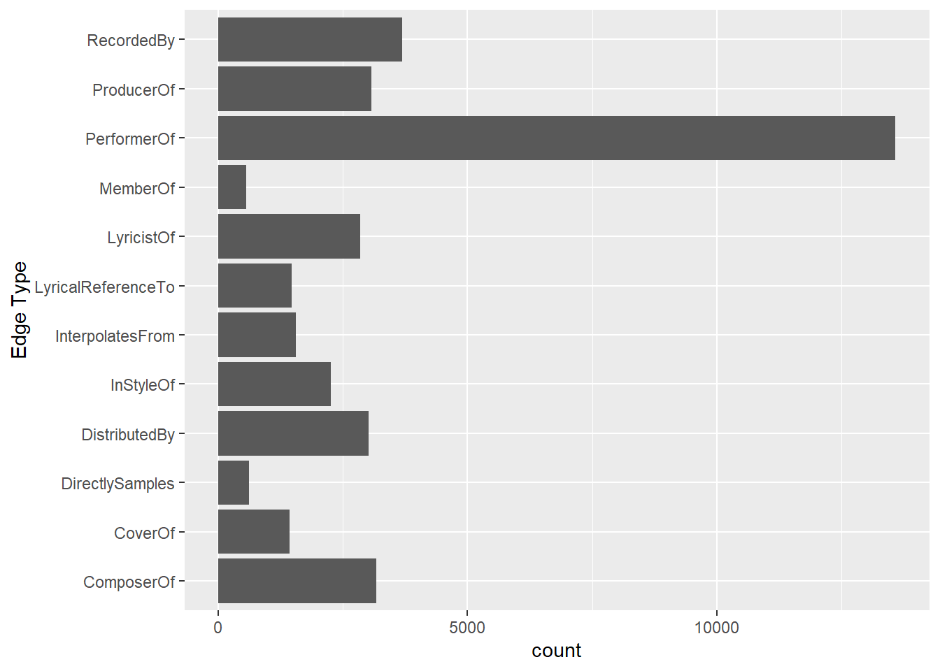
ggplot(data = mc1_nodes_clean,
       aes(y = `Node Type`)) +
  geom_bar()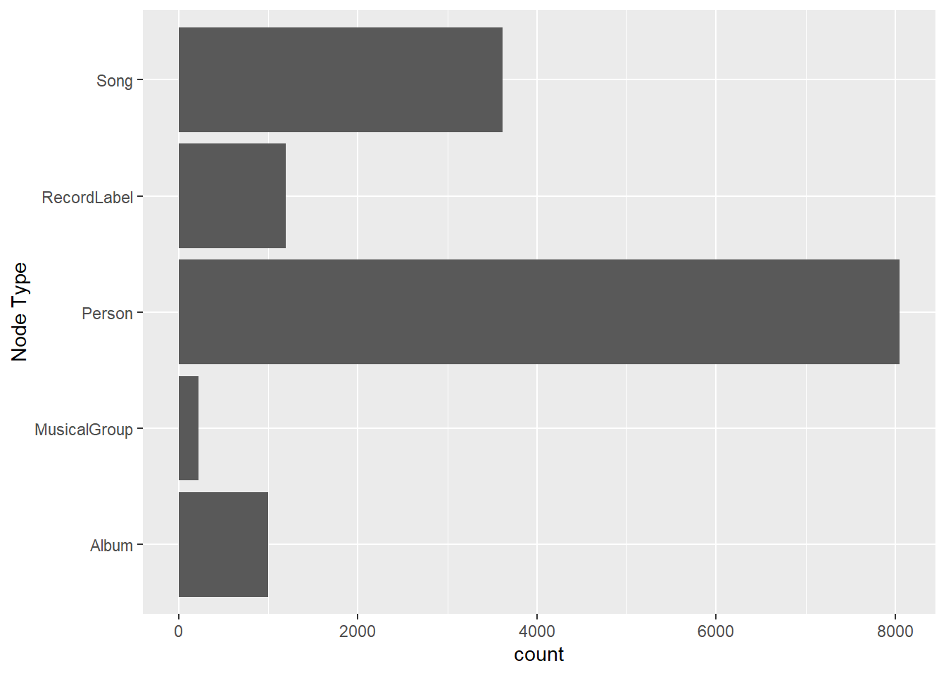
4.8 Creating knowledge graph
tbl_graph() is used to create tidygraph’s graph object by using the following code chunk.
music = tbl_graph(edges = mc1_edges_clean,
                             nodes = mc1_nodes_clean,
                             directed = TRUE)

class(music)
[1] "tbl_graph" "igraph" Several of the ggraph layouts involve randomisation. In order to ensure reproducibility, it is necessary to set the seed value before plotting by using the code chunk below.
set.seed(1234)5 VAST Challenge 2025 Mini-Challenge 1
For Task 1, it is to design and develop visualizations and visual analytic tools that will allow Silas to explore and understand the profile of Sailor Shift’s career. We start off with a network visualisation to provide an overview of Sailor Shift’s works throughout her career, as well as the various roles she played in these works.
Code
# Step 1: Identify Sailor Shift using the is_sailor column
sailor_vertex_name <- mc1_nodes_clean %>%
  filter(is_sailor) %>%
  pull(name) %>%
  first()

# Step 2: Prepare edges and nodes related to Sailor Shift
sailor_edges <- mc1_edges_clean %>%
  filter(from == sailor_vertex_name | to == sailor_vertex_name)

sailor_node_names <- unique(c(sailor_edges$from, sailor_edges$to))

sailor_nodes <- mc1_nodes_clean %>%
  filter(name %in% sailor_node_names) %>%
  distinct(name, .keep_all = TRUE)

# Step 3: Build tbl_graph object and annotate nodes
career_graph <- tbl_graph(nodes = sailor_nodes, edges = sailor_edges, directed = TRUE) %>%
  activate(nodes) %>%
  mutate(
    node_color = ifelse(is_sailor, "red", "grey30"),
    tooltip_text = paste0(
      "Name: ", node_name, "\n",
      "Type: ", `Node Type`, "\n",
      ifelse(!is.na(genre), paste0("Genre: ", genre, "\n"), ""),
      ifelse(!is.na(release_date), paste0("Release: ", release_date, "\n"), "")
    )
  )

# Step 4: Extract layout coordinates
layout_df <- create_layout(career_graph, layout = "fr") %>%
  as_tibble() %>%
  select(name, x, y)

nodes_plot <- career_graph %>%
  as_tibble() %>%
  left_join(layout_df, by = "name")

edges_plot <- sailor_edges %>%
  left_join(nodes_plot %>% select(name, x, y), by = c("from" = "name")) %>%
  rename(x_from = x, y_from = y) %>%
  left_join(nodes_plot %>% select(name, x, y), by = c("to" = "name")) %>%
  rename(x_to = x, y_to = y)

# Get Sailor Shift node coordinates for annotation
sailor_coords <- nodes_plot %>%
  filter(is_sailor) %>%
  select(x, y)

# Step 5: Plot with ggiraph
p <- ggplot() +
  # Edge layer with its own color scale
  geom_segment(
    data = edges_plot,
    aes(
      x = x_from, y = y_from, xend = x_to, yend = y_to,
      color = `Edge Type`
    ),
    alpha = 0.4, arrow = arrow(length = unit(3, 'mm'))
  ) +
  scale_color_brewer(palette = "Dark2", name = "Edge Type") +

  # New color scale for nodes
  ggnewscale::new_scale_color() +

  geom_point_interactive(
    data = nodes_plot,
    aes(
      x = x, y = y,
      tooltip = tooltip_text,
      data_id = name,
      color = node_color,
      shape = `Node Type`
    ),
    size = 4
  ) +
  scale_color_manual(
    values = c("red" = "red", "grey30" = "grey30")
  ) +
  guides(color = "none") +

  # Add Sailor Shift label in the middle of the graph
  geom_text(
    data = sailor_coords,
    aes(x = x, y = y, label = "Sailor Shift"),
    size = 6, fontface = "bold", color = "red", vjust = -1
  ) +

  theme_void() +
  labs(title = "Sailor Shift's Career Profile") +
  theme(
    plot.title = element_text(size = 16, face = "bold")
  )

girafe(ggobj = p, width_svg = 10, height_svg = 8)
Code
# Filter edges related to Sailor Shift
sailor_edges <- mc1_edges_clean %>%
  filter(from == sailor_vertex_name | to == sailor_vertex_name)

# Count edges by Edge Type
edge_counts <- sailor_edges %>%
  count(`Edge Type`) %>%
  arrange(desc(n))

# Display as a simple table
kable(edge_counts, col.names = c("Role (Edge Type)", "Count"), caption = "Sailor Shift's Career Roles")| Role (Edge Type) | Count |
|---|---|
| PerformerOf | 26 |
| LyricistOf | 21 |
| MemberOf | 1 |
| ProducerOf | 1 |
Code
# Filter edges related to Sailor Shift
sailor_edges <- mc1_edges_clean %>%
  filter(from == sailor_vertex_name | to == sailor_vertex_name)

# Get the names of nodes connected to Sailor Shift
related_names <- unique(c(sailor_edges$from, sailor_edges$to))
related_names <- setdiff(related_names, sailor_vertex_name)

# Get node types for these connected nodes
related_nodes <- mc1_nodes_clean %>%
  filter(name %in% related_names)

# Count by Node Type (Song, Album)
type_counts <- related_nodes %>%
  filter(`Node Type` %in% c("Song", "Album")) %>%
  count(`Node Type`) %>%
  arrange(desc(n))

# Display as a simple table
kable(type_counts, col.names = c("Type", "Count"), caption = "Number of Songs and Albums Related to Sailor Shift")| Type | Count |
|---|---|
| Album | 21 |
| Song | 17 |
Based on the above, Sailor Shift is primarily a performer and lyricist, and a member of Ivy Echos, a musical group. Her works consist of 21 albums and 17 songs. It also shows that Oceanic Records, a Record label, has participated in the production of her works.
5.1 Question 1a - Who has she been most influenced by over time?
The network structure below shows how Sailor Shift’s career has been influenced by others. PageRank is used to measure the overall influence of each person, musical group or work within the network. This captures both direct and indirect influences.
Code
# Step 0: Get name of 'Sailor Shift'
sailor_vertex_name <- mc1_nodes_clean %>%
  filter(is_sailor == TRUE) %>%
  pull(name) %>%
  first()

# Step 1: Find direct influence relationships from Sailor Shift
# These are the artists/works that Sailor Shift has been influenced by
direct_influence_types <- c("InStyleOf", "CoverOf", "InterpolatesFrom", "LyricalReferenceTo", "DirectlySamples")

sailor_direct_influences <- mc1_edges_clean %>%
  filter(from == sailor_vertex_name,
         `Edge Type` %in% direct_influence_types)

# Step 2: Get immediate neighbors (people/groups Sailor Shift works with)
sailor_out_edges <- mc1_edges_clean %>%
  filter(from == sailor_vertex_name)

sailor_out_node_names <- sailor_out_edges$to

# Step 3: Split into people/groups vs songs/albums
sailor_person_group <- mc1_nodes_clean %>%
  filter(name %in% sailor_out_node_names, `Node Type` %in% c("Person", "MusicalGroup")) %>%
  pull(name)

sailor_songs_all <- mc1_nodes_clean %>%
  filter(name %in% sailor_out_node_names, `Node Type` %in% c("Song", "Album")) %>%
  pull(name)

# Step 4: For songs/albums, find their direct influences too
song_influences <- mc1_edges_clean %>%
  filter(from %in% sailor_songs_all,
         `Edge Type` %in% direct_influence_types)

# Step 5: Get all influence targets (who influenced Sailor Shift or their works)
all_influence_targets <- unique(c(
  sailor_direct_influences$to,
  song_influences$to
))

# Step 6: Get creators of Sailor Shift's works (indirect influence indicators)
creator_edge_types <- c("PerformerOf", "ComposerOf", "ProducerOf", "LyricistOf")

sailor_songs <- mc1_edges_clean %>%
  filter(from %in% sailor_songs_all) %>%
  pull(from) %>%
  unique()

sailor_songs_out_nodes <- mc1_edges_clean %>%
  filter(from %in% sailor_songs) %>%
  pull(to)

creator_edges <- mc1_edges_clean %>%
  filter(to %in% sailor_songs_out_nodes, `Edge Type` %in% creator_edge_types)

sailor_people_group_neighbourhood_nodes <- creator_edges %>%
  pull(from) %>%
  unique()

# Step 7: Combine all relevant nodes for subgraph
sailor_all_node_names <- unique(c(
  sailor_vertex_name,
  sailor_person_group,
  sailor_songs,
  sailor_songs_out_nodes,
  sailor_people_group_neighbourhood_nodes,
  all_influence_targets
))

# Step 8: Create subgraph
sub_music <- music %>%
  filter(name %in% sailor_all_node_names)

# Step 9: Calculate PageRank
sub_music <- sub_music %>%
  activate(nodes) %>%
  mutate(
    pagerank = centrality_pagerank()
  )

# Step 10: Set node size based on PageRank for people/groups, fixed for others
sub_music <- sub_music %>%
  mutate(
    is_sailor = name == sailor_vertex_name,
    node_color = ifelse(is_sailor, "red", "grey30"),
    tooltip_text = sprintf(
      "Name: %s\nType: %s\nPageRank: %.4f",
      node_name, `Node Type`, pagerank
    ),
    node_size = case_when(
      `Node Type` %in% c("Person", "MusicalGroup") ~ rescale(pagerank, to = c(4, 20)),
      TRUE ~ 4
    )
  )

# Step 11: Create visualization
g <- sub_music %>%
  ggraph(layout = "fr") +
  geom_edge_link(
    aes(color = `Edge Type`),
    alpha = 0.3,
    arrow = arrow(length = unit(3, 'mm')),
    end_cap = circle(3, 'mm')
  ) +
  geom_point_interactive(
    aes(
      x = x, y = y,
      data_id = name,
      tooltip = tooltip_text,
      shape = `Node Type`,
      colour = node_color,
      size = node_size
    )
  ) +
  scale_shape_discrete(name = "Node Type") +
  scale_colour_identity() +
  scale_size_identity() +
  theme_graph(base_family = "sans") +
  labs(
    title = "Network of Influences on Sailor Shift"
  )

girafe(ggobj = g, width_svg = 10, height_svg = 8)
Code
# Filter to people and groups only, exclude Sailor Shift node itself
top_influencers <- sub_music %>%
  as_tibble() %>%
  filter(
    `Node Type` %in% c("Person", "MusicalGroup"),
    name != sailor_vertex_name
  ) %>%
  arrange(desc(pagerank)) %>%
  slice_head(n = 5)

# Plot
ggplot(top_influencers, aes(x = reorder(node_name, pagerank), y = pagerank, fill = `Node Type`)) +
  geom_bar(stat = "identity") +
  coord_flip() +
  labs(
    title = "Top 5 Influences on Sailor Shift",
    x = "Influencer",
    y = "PageRank Score"
  ) +
  theme_minimal()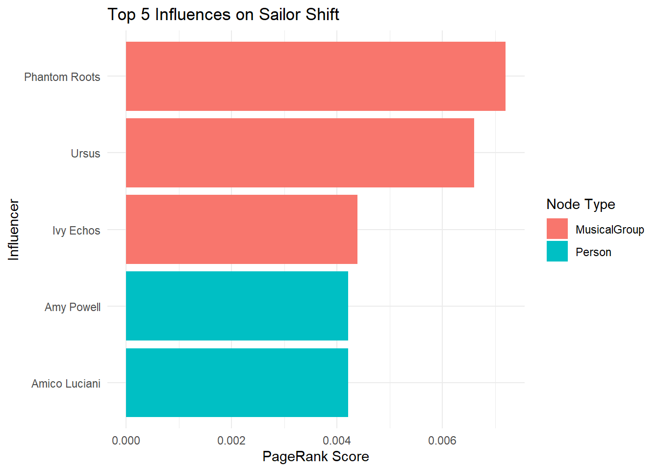
Based on the PageRank score, it is noted that she is most influenced by musical groups as the top 3 most influences are musical groups. Phantom Roots have influenced her the most over time, this is followed by Ursus and the group she was a part of, Ivy Echos.
5.2 Question 1b - Who has she collaborated with and directly or indirectly influenced?
The network visualisation below explores Sailor Shift’s collaborations and influence. While the primary question centers on Sailor Shift, the analysis also incorporates Ivy Echos, the musical group that she was a member of. Including Ivy Echos is essential because Sailor Shift’s creative impact can extend beyond her solo work as her contributions as part of Ivy Echos could have influenced others. The visualisation therefore highlights not just individuals and groups who have collaborated with Sailor Shift on her works, but also those influenced by Ivy Echos, providing an extensive picture of her influence.
Code
# Step 1: Define all relevant edge types per schema
collab_credit_types <- c("PerformerOf", "ComposerOf", "ProducerOf", "LyricistOf", "MemberOf")
influence_types <- c("CoverOf", "InterpolatesFrom", "LyricalReferenceTo", "DirectlySamples", "InStyleOf")

# Step 2: Get Sailor Shift's node ID
sailor_vertex_name <- mc1_nodes_clean %>%
  filter(is_sailor == TRUE) %>%
  pull(name) %>% first()

# Step 3: Find all Sailor Shift's works (songs/albums she performed or was lyricist of)
sailor_works <- mc1_edges_clean %>%
  filter(`Edge Type` %in% c("PerformerOf", "LyricistOf"), from == sailor_vertex_name) %>%
  pull(to)

# Step 4: Find all Person/MusicalGroup collaborated on Sailor Shift's works (excluding herself)
sailor_collab_edges <- mc1_edges_clean %>%
  filter(`Edge Type` %in% collab_credit_types, to %in% sailor_works, from != sailor_vertex_name)
sailor_collab_nodes <- mc1_nodes_clean %>%
  filter(name %in% sailor_collab_edges$from, `Node Type` %in% c("Person", "MusicalGroup")) %>%
  pull(name)

# Step 5: Get Ivy Echos's node ID and works
ivy_echos_name <- mc1_nodes_clean %>%
  filter(str_detect(node_name, regex("Ivy Echos", ignore_case = TRUE))) %>%
  pull(name) %>% first()
ivy_works <- mc1_edges_clean %>%
  filter(`Edge Type` == "PerformerOf", from == ivy_echos_name) %>%
  pull(to)
ivy_works <- mc1_nodes_clean %>%
  filter(name %in% ivy_works, `Node Type` %in% c("Song", "Album")) %>%
  pull(name)

# Step 6: Find all works influenced by Ivy Echos's works (Ivy Echos's works as destination of influence edges)
ivy_influenced_edges <- mc1_edges_clean %>%
  filter(`Edge Type` %in% influence_types, to %in% ivy_works)
ivy_influenced_works <- ivy_influenced_edges$from

# Step 7: For each influenced work, get the people/groups involved (collaborators on those works)
ivy_influenced_collab_edges <- mc1_edges_clean %>%
  filter(`Edge Type` %in% collab_credit_types, to %in% ivy_influenced_works)
ivy_influenced_collab_nodes <- mc1_nodes_clean %>%
  filter(name %in% ivy_influenced_collab_edges$from, `Node Type` %in% c("Person", "MusicalGroup")) %>%
  pull(name)

# Step 8: Collect all relevant nodes and edges for the network
all_relevant_nodes <- unique(c(
  sailor_vertex_name,
  sailor_collab_nodes,
  sailor_works,
  ivy_echos_name,
  ivy_works,
  ivy_influenced_works,
  ivy_influenced_collab_nodes
))

all_relevant_edges <- mc1_edges_clean %>%
  filter(from %in% all_relevant_nodes & to %in% all_relevant_nodes)

# Step 9: Annotate node roles for plotting
sub_nodes_df <- mc1_nodes_clean %>%
  filter(name %in% all_relevant_nodes) %>%
  mutate(
    node_role = case_when(
      name == sailor_vertex_name ~ "Sailor Shift",
      name == ivy_echos_name ~ "Ivy Echos",
      name %in% sailor_collab_nodes ~ "Sailor Shift Collaborator",
      name %in% sailor_works ~ "Sailor Shift Work",
      name %in% ivy_works ~ "Ivy Echos Work",
      name %in% ivy_influenced_works ~ "Work Influenced by Ivy Echos",
      name %in% ivy_influenced_collab_nodes ~ "Person/Group in Influenced Work",
      TRUE ~ "Other"
    ),
    node_color = case_when(
      node_role == "Sailor Shift" ~ "red",
      node_role == "Ivy Echos" ~ "purple",
      node_role == "Sailor Shift Collaborator" ~ "blue",
      node_role == "Sailor Shift Work" ~ "grey30",
      node_role == "Ivy Echos Work" ~ "green",
      node_role == "Work Influenced by Ivy Echos" ~ "orange",
      node_role == "Person/Group in Influenced Work" ~ "pink",
      TRUE ~ "steelblue"
    ),
    tooltip_text = paste0(
      "Name: ", node_name, "\n",
      "Type: ", `Node Type`, "\n",
      "Role: ", node_role, "\n",
      ifelse(!is.na(genre), paste0("Genre: ", genre, "\n"), ""),
      ifelse(!is.na(release_date), paste0("Release: ", release_date, "\n"), "")
    )
  )

# Step 10: Create tidygraph object and layout
career_graph <- tbl_graph(nodes = sub_nodes_df, edges = all_relevant_edges, directed = TRUE) %>%
  activate(nodes)

layout_df <- create_layout(career_graph, layout = "fr") %>%
  as_tibble() %>%
  select(name, x, y)

nodes_plot <- as_tibble(career_graph) %>%
  left_join(layout_df, by = "name")

edges_plot <- all_relevant_edges %>%
  left_join(nodes_plot %>% select(name, x, y), by = c("from" = "name")) %>%
  rename(x_from = x, y_from = y) %>%
  left_join(nodes_plot %>% select(name, x, y), by = c("to" = "name")) %>%
  rename(x_to = x, y_to = y)

# Step 11: Get coordinates for annotation
sailor_coords <- nodes_plot %>%
  filter(name == sailor_vertex_name) %>%
  select(x, y)
ivy_coords <- nodes_plot %>%
  filter(name == ivy_echos_name) %>%
  select(x, y)

# Step 12: Plot with ggplot2 + ggiraph, with annotation and legend
p <- ggplot() +
  geom_segment(
    data = edges_plot,
    aes(
      x = x_from, y = y_from, xend = x_to, yend = y_to,
      color = `Edge Type`
    ),
    alpha = 0.4, arrow = arrow(length = unit(3, 'mm'))
  ) +
  scale_color_brewer(palette = "Dark2", name = "Edge Type") +
  ggnewscale::new_scale_color() +
  geom_point_interactive(
    data = nodes_plot,
    aes(
      x = x, y = y,
      tooltip = tooltip_text,
      data_id = name,
      color = node_role,
      shape = `Node Type`
    ),
    size = 4
  ) +
  scale_color_manual(
    name = "Node Role",
    values = c(
      "Sailor Shift" = "red",
      "Ivy Echos" = "purple",
      "Sailor Shift Collaborator" = "blue",
      "Sailor Shift Work" = "grey30",
      "Ivy Echos Work" = "green",
      "Work Influenced by Ivy Echos" = "orange",
      "Person/Group in Influenced Work" = "pink",
      "Other" = "steelblue"
    ),
    breaks = c(
      "Sailor Shift",
      "Ivy Echos",
      "Sailor Shift Collaborator",
      "Sailor Shift Work",
      "Ivy Echos Work",
      "Work Influenced by Ivy Echos",
      "Person/Group in Influenced Work"
    )
  ) +
  theme_void() +
  labs(title = "Sailor Shift's Collaborators and Influence") +
  guides(
    color = guide_legend(
      title = "Node Role",
      override.aes = list(size = 4),
      title.position = "top"
    ),
    shape = guide_legend(
      title = "Node Type",
      title.position = "top"
    )
  ) +
  theme(
    legend.position = "right",
    legend.box = "vertical",
    plot.title = element_text(size = 20, face = "bold")
  )

girafe(ggobj = p, width_svg = 12, height_svg = 8)
The visualisation shows a wide array of individuals and musical groups who have collaborated with Sailor Shift on various works, this reflects her active engagement within the industry. While there are no instances of Sailor Shift directly influencing other artists, the visualisation reveals that her group, Ivy Echos, has influenced a group and four individuals through a song (Deepsea Fireflies, released in 2025). This demonstrates that Sailor Shift’s reach extends beyond her personal collaborations, contributing to a broader legacy through her involvement with Ivy Echos.
5.3 Question 1c - How has she influenced collaborators of the broader Oceanus Folk community?
The network visualisation aims to analyse how Sailor Shift influenced collaborators of the broader Oceanus Folk community.
Sailor Shift and her group (Ivy Echos) were primary entities of interest, all works associated to them are compiled to form the foundation of Sailor Shift’s musical output. Based on this, several types of influence were analysed:
- Direct influence - This includes Oceanus Folk collaborators’ works that were explicity influenced by Sailor Shift or Ivy Echos through relationships such as CoverOf, InterpolatesFrom, LyricalReferenceTo, DirectlySamples, and InStyleOf.
- Indirect (two-step influence) - This occurs when a work by Sailor Shift or Ivy Echos influences an intermediate piece, which then goes on to influence a work by an Oceanus Folk collaborator. These two-step chains shows how Sailor Shift’s influence can propagate through the network.
- Cross-collaborator influence - This captures intra-community influence where Oceanus Folk works that were initially influenced by Sailor Shift/Ivy Echos proceeded to influence other Oceanus Folk creations.
- Collaboration-mediated influence - This is transmitted through shared or bridge collaborators.
- Shared collaborators are individuals or groups who worked with both Sailor Shift/Ivy Echos and the Oceanus Folk community
- Bridge Collaborators are those who first worked with Sailor Shift/Ivy Echos and later collaborated with Ocean Folk Contributors.
Based on the influences above, it reveals the full extent of Sailor Shift’s reach within the Oceanus Folk Community.
Code
# Step 1: Define edge types
collab_credit_types <- c("PerformerOf", "ComposerOf", "ProducerOf", "LyricistOf", "MemberOf")
influence_edge_types <- c("CoverOf", "InterpolatesFrom", "LyricalReferenceTo", "DirectlySamples", "InStyleOf")

# Step 2: Identify all nodes with genre == "Oceanus Folk"
oceanus_folk_works <- mc1_nodes_clean %>%
  filter(genre == "Oceanus Folk") %>%
  pull(name)

# Step 3: Identify all Person and MusicalGroup who are collaborators on Oceanus Folk works
oceanus_folk_collaborators <- mc1_edges_clean %>%
  filter(`Edge Type` %in% collab_credit_types,
         to %in% oceanus_folk_works) %>%
  inner_join(mc1_nodes_clean %>% select(name, `Node Type`), by = c("from" = "name")) %>%
  filter(`Node Type` %in% c("Person", "MusicalGroup")) %>%
  pull(from) %>%
  unique()

# Step 4: Get Sailor Shift and Ivy Echos
sailor_vertex_name <- mc1_nodes_clean %>%
  filter(is_sailor == TRUE) %>%
  pull(name) %>%
  first()

ivy_echos_name <- mc1_edges_clean %>%
  filter(`Edge Type` == "MemberOf", from == sailor_vertex_name) %>%
  pull(to) %>%
  first()

# Step 5: Find all works that Sailor Shift and Ivy Echos have created/performed
sailor_works <- mc1_edges_clean %>%
  filter(`Edge Type` %in% collab_credit_types, from == sailor_vertex_name) %>%
  pull(to)

ivy_works <- mc1_edges_clean %>%
  filter(`Edge Type` %in% collab_credit_types, from == ivy_echos_name) %>%
  pull(to)

sailor_ivy_works <- unique(c(sailor_works, ivy_works))

# Step 6: Find all works that the Oceanus Folk collaborators have worked on
oceanus_collaborator_works <- mc1_edges_clean %>%
  filter(`Edge Type` %in% collab_credit_types,
         from %in% oceanus_folk_collaborators) %>%
  pull(to) %>%
  unique()

# Step 7: Direct influence - Sailor Shift/Ivy Echos works influencing Oceanus collaborator works
direct_influence <- mc1_edges_clean %>%
  filter(`Edge Type` %in% influence_edge_types,
         from %in% sailor_ivy_works,
         to %in% oceanus_collaborator_works) %>%
  mutate(influence_direction = "Sailor/Ivy → Oceanus",
         pathway_type = "Direct")

# Step 8: Indirect influence - Multi-step pathways

# 8a: Find intermediate works that could bridge Sailor Shift/Ivy Echos to Oceanus
# Works influenced BY Sailor/Ivy
sailor_influenced_works <- mc1_edges_clean %>%
  filter(`Edge Type` %in% influence_edge_types,
         from %in% sailor_ivy_works) %>%
  pull(to) %>%
  unique()

# Works that influence Sailor/Ivy
sailor_influencing_works <- mc1_edges_clean %>%
  filter(`Edge Type` %in% influence_edge_types,
         to %in% sailor_ivy_works) %>%
  pull(from) %>%
  unique()

# All intermediate works in potential pathways
intermediate_works <- unique(c(sailor_influenced_works, sailor_influencing_works))

# 8b: Two-step influence: Sailor/Ivy → Intermediate → Oceanus collaborators
indirect_influence_step1 <- mc1_edges_clean %>%
  filter(`Edge Type` %in% influence_edge_types,
         from %in% sailor_ivy_works,
         to %in% intermediate_works) %>%
  select(sailor_work = from, intermediate_work = to, step1_edge_type = `Edge Type`)

indirect_influence_step2 <- mc1_edges_clean %>%
  filter(`Edge Type` %in% influence_edge_types,
         from %in% intermediate_works,
         to %in% oceanus_collaborator_works) %>%
  select(intermediate_work = from, oceanus_work = to, step2_edge_type = `Edge Type`)

# Join to find complete 2-step pathways
two_step_pathways <- indirect_influence_step1 %>%
  inner_join(indirect_influence_step2, by = "intermediate_work") %>%
  mutate(pathway_type = "Indirect (2-step)",
         influence_direction = "Sailor/Ivy → Intermediate → Oceanus")

# 8c: Cross-collaborator influence within Oceanus community
# Find Oceanus works that were influenced by Sailor and then influenced other Oceanus works
directly_influenced_oceanus_works <- unique(c(direct_influence$to, two_step_pathways$oceanus_work))

cross_collab_influence <- mc1_edges_clean %>%
  filter(`Edge Type` %in% influence_edge_types,
         from %in% directly_influenced_oceanus_works,
         to %in% oceanus_collaborator_works,
         from != to) %>%
  mutate(pathway_type = "Cross-collaborator",
         influence_direction = "Sailor-influenced Oceanus work → Other Oceanus work")

# Step 9: Collaboration-mediated influence

# 9a: People who worked with both Sailor/Ivy AND Oceanus Folk collaborators
sailor_ivy_collaborators <- mc1_edges_clean %>%
  filter(`Edge Type` %in% collab_credit_types,
         to %in% sailor_ivy_works) %>%
  inner_join(mc1_nodes_clean %>% select(name, `Node Type`), by = c("from" = "name")) %>%
  filter(`Node Type` %in% c("Person", "MusicalGroup")) %>%
  pull(from) %>%
  unique()

shared_collaborators <- intersect(sailor_ivy_collaborators, oceanus_folk_collaborators)

# 9b. Bridge collaborators - worked with Sailor/Ivy, then later with other Oceanus Folk collaborators
bridge_collaborators <- setdiff(sailor_ivy_collaborators, oceanus_folk_collaborators)
bridge_to_oceanus <- mc1_edges_clean %>%
  filter(`Edge Type` %in% collab_credit_types,
         from %in% bridge_collaborators) %>%
  inner_join(
    mc1_edges_clean %>%
      filter(`Edge Type` %in% collab_credit_types,
             from %in% oceanus_folk_collaborators) %>%
      select(shared_work = to),
    by = c("to" = "shared_work")
  ) %>%
  select(bridge_person = from, shared_work = to) %>%
  distinct()

# Step 10: Identify influenced Oceanus Folk Collaborators

# Get all works that show influence from Sailor/Ivy
all_influenced_oceanus_works <- unique(c(
  direct_influence$to,
  two_step_pathways$oceanus_work,
  cross_collab_influence$to
))

# Find which Oceanus Folk collaborators worked on these influenced works
directly_influenced_collaborators <- mc1_edges_clean %>%
  filter(`Edge Type` %in% collab_credit_types,
         to %in% all_influenced_oceanus_works) %>%
  inner_join(mc1_nodes_clean %>% select(name, `Node Type`), by = c("from" = "name")) %>%
  filter(`Node Type` %in% c("Person", "MusicalGroup"),
         from %in% oceanus_folk_collaborators) %>%
  pull(from) %>%
  unique()

# Add collaborators connected through shared/bridge relationships
collaboration_influenced <- unique(c(shared_collaborators, bridge_to_oceanus$bridge_person))
collaboration_influenced <- intersect(collaboration_influenced, oceanus_folk_collaborators)

total_influenced_collaborators <- unique(c(directly_influenced_collaborators, collaboration_influenced))

# Prepare variables for tabset (initialize as NULL)
p <- NULL
summary_stats <- NULL

# Step 11: Enhanced network visualisation and summary statistics
if(length(total_influenced_collaborators) > 0) {

  # Collect all relevant nodes for visualization
  all_pathway_works <- unique(c(
    sailor_ivy_works,
    direct_influence$from, direct_influence$to,
    two_step_pathways$sailor_work, two_step_pathways$intermediate_work, two_step_pathways$oceanus_work,
    cross_collab_influence$from, cross_collab_influence$to
  ))

  all_relevant_people <- unique(c(
    sailor_vertex_name,
    ivy_echos_name,
    total_influenced_collaborators,
    shared_collaborators,
    bridge_to_oceanus$bridge_person
  ))

  all_viz_nodes <- unique(c(all_pathway_works, all_relevant_people))

  # Enhanced node classification
  viz_nodes <- mc1_nodes_clean %>%
    filter(name %in% all_viz_nodes) %>%
    mutate(
      influence_strength = case_when(
        name %in% direct_influence$to ~ "Direct Target",
        name %in% two_step_pathways$oceanus_work ~ "Indirect Target",
        name %in% cross_collab_influence$to ~ "Secondary Target",
        name %in% shared_collaborators ~ "Shared Collaborator",
        name %in% bridge_to_oceanus$bridge_person ~ "Bridge Collaborator",
        TRUE ~ "Network Node"
      ),
      node_role = case_when(
        name == sailor_vertex_name ~ "Sailor Shift",
        name == ivy_echos_name ~ "Ivy Echos",
        name %in% sailor_ivy_works ~ "Sailor/Ivy Work",
        name %in% oceanus_folk_works ~ "Oceanus Folk Work",
        name %in% total_influenced_collaborators ~ "Influenced Oceanus Collaborator",
        name %in% oceanus_folk_collaborators ~ "Other Oceanus Collaborator",
        name %in% intermediate_works ~ "Intermediate Work",
        TRUE ~ "Other"
      ),
      node_color = case_when(
        node_role == "Sailor Shift" ~ "red",
        node_role == "Ivy Echos" ~ "purple",
        node_role == "Sailor/Ivy Work" ~ "gray30",
        influence_strength == "Direct Target" ~ "darkred",
        influence_strength == "Indirect Target" ~ "orange",
        influence_strength == "Secondary Target" ~ "yellow",
        influence_strength == "Shared Collaborator" ~ "blue",
        influence_strength == "Bridge Collaborator" ~ "cyan",
        node_role == "Influenced Oceanus Collaborator" ~ "darkgreen",
        node_role == "Other Oceanus Collaborator" ~ "lightgreen",
        node_role == "Intermediate Work" ~ "pink",
        TRUE ~ "lightgray"
      ),
      node_size = case_when(
        node_role %in% c("Sailor Shift", "Ivy Echos") ~ 8,
        influence_strength %in% c("Direct Target", "Shared Collaborator") ~ 6,
        influence_strength %in% c("Indirect Target", "Bridge Collaborator") ~ 5,
        influence_strength == "Secondary Target" ~ 4,
        TRUE ~ 3
      ),
      tooltip_text = paste0(
        "Name: ", node_name, "\n",
        "Role: ", node_role, "\n",
        "Influence: ", influence_strength, "\n",
        "Type: ", `Node Type`, "\n",
        ifelse(!is.na(genre), paste0("Genre: ", genre), "")
      )
    )

  # Collect all relevant edges preserving original Edge Types
  all_influence_edges <- bind_rows(
    direct_influence %>% mutate(pathway_category = "Direct"),
    two_step_pathways %>%
      select(from = sailor_work, to = intermediate_work, `Edge Type` = step1_edge_type) %>%
      mutate(pathway_category = "Indirect Step 1"),
    two_step_pathways %>%
      select(from = intermediate_work, to = oceanus_work, `Edge Type` = step2_edge_type) %>%
      mutate(pathway_category = "Indirect Step 2"),
    cross_collab_influence %>%
      select(from, to, `Edge Type`) %>%
      mutate(pathway_category = "Cross-Collaborator")
  )

  viz_edges <- mc1_edges_clean %>%
    filter(from %in% all_viz_nodes, to %in% all_viz_nodes) %>%
    left_join(
      all_influence_edges %>% select(from, to, pathway_category),
      by = c("from", "to")
    ) %>%
    mutate(
      # Categorize edges for visual emphasis while keeping original Edge Type
      edge_category = case_when(
        !is.na(pathway_category) ~ "Influence Pathway",
        `Edge Type` == "MemberOf" & from == sailor_vertex_name ~ "Key Membership",
        `Edge Type` %in% collab_credit_types ~ "Collaboration",
        `Edge Type` %in% influence_edge_types ~ "Other Influence",
        TRUE ~ "Other"
      ),
      edge_alpha = case_when(
        edge_category == "Influence Pathway" ~ 0.9,
        edge_category == "Key Membership" ~ 0.8,
        edge_category == "Collaboration" ~ 0.4,
        edge_category == "Other Influence" ~ 0.6,
        TRUE ~ 0.2
      )
    )

  # Create network plot
  influence_graph <- tbl_graph(nodes = viz_nodes, edges = viz_edges, directed = TRUE)

  layout_df <- create_layout(influence_graph, layout = "fr") %>%
    as_tibble() %>%
    select(name, x, y)

  nodes_plot <- as_tibble(influence_graph) %>%
    left_join(layout_df, by = "name")

  edges_plot <- viz_edges %>%
    left_join(nodes_plot %>% select(name, x, y), by = c("from" = "name")) %>%
    rename(x_from = x, y_from = y) %>%
    left_join(nodes_plot %>% select(name, x, y), by = c("to" = "name")) %>%
    rename(x_to = x, y_to = y)

  # Create legend data frame for node colors
  legend_data <- data.frame(
    node_color = c("red", "purple", "gray30", "darkred", "orange", "yellow",
                   "blue", "cyan", "darkgreen", "lightgreen", "pink", "lightgray"),
    node_role = c("Sailor Shift", "Ivy Echos", "Sailor/Ivy Work", "Direct Target",
                  "Indirect Target", "Secondary Target", "Shared Collaborator",
                  "Bridge Collaborator", "Influenced Oceanus Collaborator",
                  "Other Oceanus Collaborator", "Intermediate Work", "Other"),
    stringsAsFactors = FALSE
  )

  p <- ggplot() +
    geom_segment(
      data = edges_plot,
      aes(x = x_from, y = y_from, xend = x_to, yend = y_to,
          color = `Edge Type`, alpha = edge_alpha),
      arrow = arrow(length = unit(1.5, 'mm'))
    ) +
    scale_alpha_identity() +
    scale_color_discrete(name = "Edge Type") +
    ggnewscale::new_scale_color() +
    geom_point_interactive(
      data = nodes_plot,
      aes(x = x, y = y, tooltip = tooltip_text, data_id = name,
          color = node_color, shape = `Node Type`, size = node_size)
    ) +
    scale_size_identity() +
    scale_color_manual(
      name = "Node Role",
      values = c("red" = "red", "purple" = "purple", "pink" = "pink", "darkred" = "darkred",
                 "orange" = "orange", "yellow" = "yellow", "blue" = "blue", "cyan" = "cyan",
                 "darkgreen" = "darkgreen", "lightgreen" = "lightgreen",
                 "gray30" = "gray30", "lightgray" = "lightgray"),
      labels = setNames(legend_data$node_role, legend_data$node_color),
      breaks = legend_data$node_color,
      guide = guide_legend(override.aes = list(size = 4, shape = 16))
    ) +
    geom_text(
      data = nodes_plot %>% filter(node_role == "Sailor Shift"),
      aes(x = x, y = y, label = "Sailor Shift"),
      size = 4, fontface = "bold", color = "red", vjust = -2
    ) +
    theme_void() +
    theme(
      legend.position = "right",
      legend.box = "vertical",
      legend.text = element_text(size = 11),
      legend.title = element_text(size = 16),
      plot.title = element_text(size = 20, face = "bold"),
      plot.subtitle = element_text(size = 16, face = "plain")
    ) +
    labs(
      title = "Sailor Shift's Influence on Oceanus Folk Community",
      subtitle = str_to_title("Influence pathways: Direct (work-to-work), Indirect (via intermediary), Secondary (cross-collaborator), Shared/Bridge (collaboration networks)")
    )

  # Create summary statistics data frame
summary_stats <- data.frame(
  Metric = c(
    "Total Oceanus Folk collaborators",
    "Total influenced collaborators",
    "Percentage influenced (%)",
    "",
    "Direct influences",
    "Two-step pathways",
    "Cross-collaborator influences",
    "Shared collaborators",
    "Bridge collaborators"
  ),
  Value = c(
    length(oceanus_folk_collaborators),
    length(total_influenced_collaborators),
    round(100 * length(total_influenced_collaborators) / length(oceanus_folk_collaborators), 1),
    "",
    nrow(direct_influence),
    nrow(two_step_pathways),
    nrow(cross_collab_influence),
    length(shared_collaborators),
    length(unique(bridge_to_oceanus$bridge_person))
  ),
  stringsAsFactors = FALSE
)
}Code
girafe(ggobj = p, width_svg = 16, height_svg = 12)Code
knitr::kable(
  summary_stats,
  col.names = c("Metric", "Count"),
  caption = "Sailor Shift's Influence Analysis Summary"
)| Metric | Count |
|---|---|
| Total Oceanus Folk collaborators | 720 |
| Total influenced collaborators | 81 |
| Percentage influenced (%) | 11.2 |
| Direct influences | 9 |
| Two-step pathways | 11 |
| Cross-collaborator influences | 10 |
| Shared collaborators | 42 |
| Bridge collaborators | 7 |
The above visualisation focus on the network of influence that Sailor Shift had in the Oceanus Folk community. Out of 720 Oceanus Folk collaborators, she has interacted with 81 collaborators, which is a notable influence as it is more than 10% of the community.
While only 9 collaborators have been directly influenced by working closely with her/Ivy Echos, the majority of her impact is indirect. More than half of the influenced collaborators have been shaped indirectly through shared and bridged collaborators. These network-mediated pathways, including two-step and cross-collaborator connections, illustrates how her influence extends beyond those that she worked directly with.
Overall, this showcases how Sailor Shift’s influence diffuses dynamically throughout the community where her impact in the community is not only driven by direct collaborations, but also by the broader web of relationships and interactions that connect the Oceanus Folk community.